Area lights in shaders [work notes]

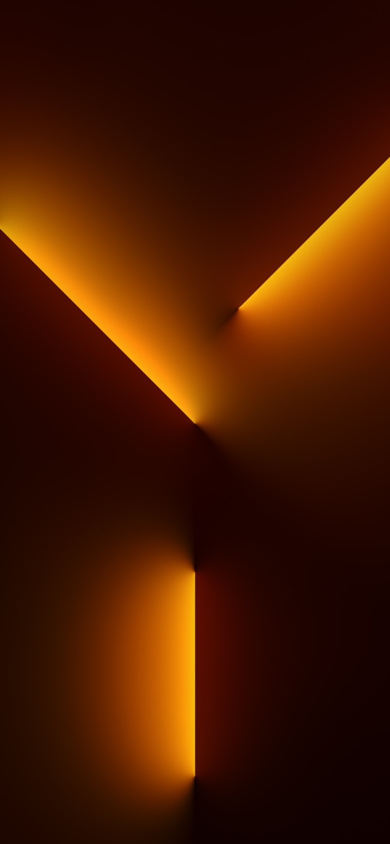
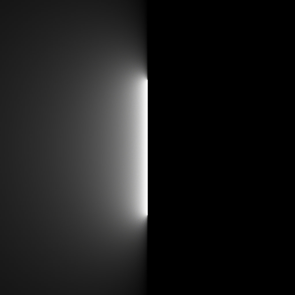
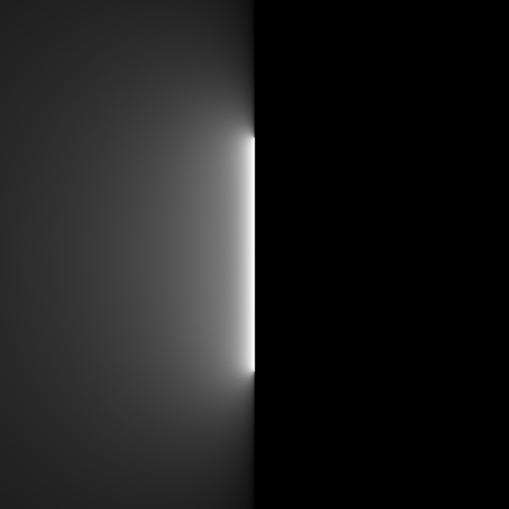
I'm trying to recreate the 2D area light effect from the iPhone 13 wallpapers in GLSL pixel shaders.

This is a "work notes" blog post I'm writing as I learn, I'll definitely make mistakes while I do so. If you have some corrections, feel free to DM me on Twitter or email me.

Analysing reference image

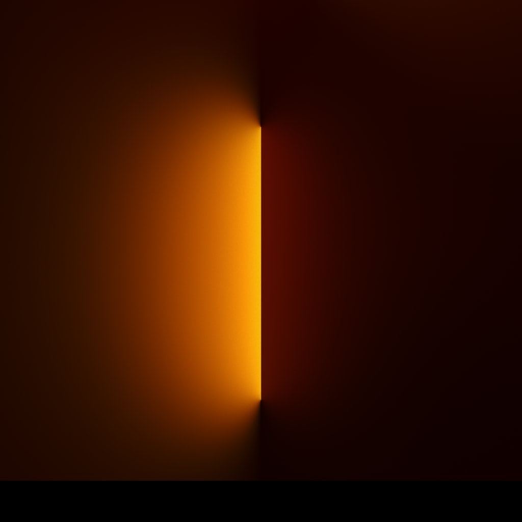
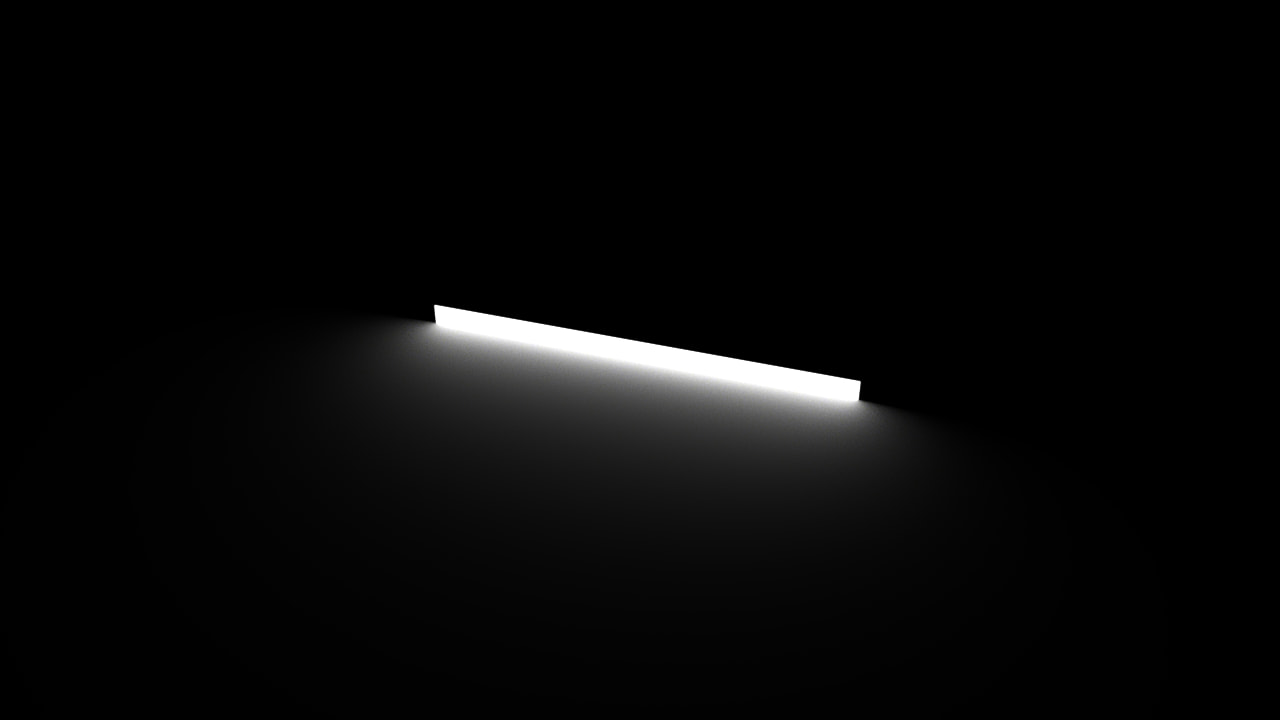
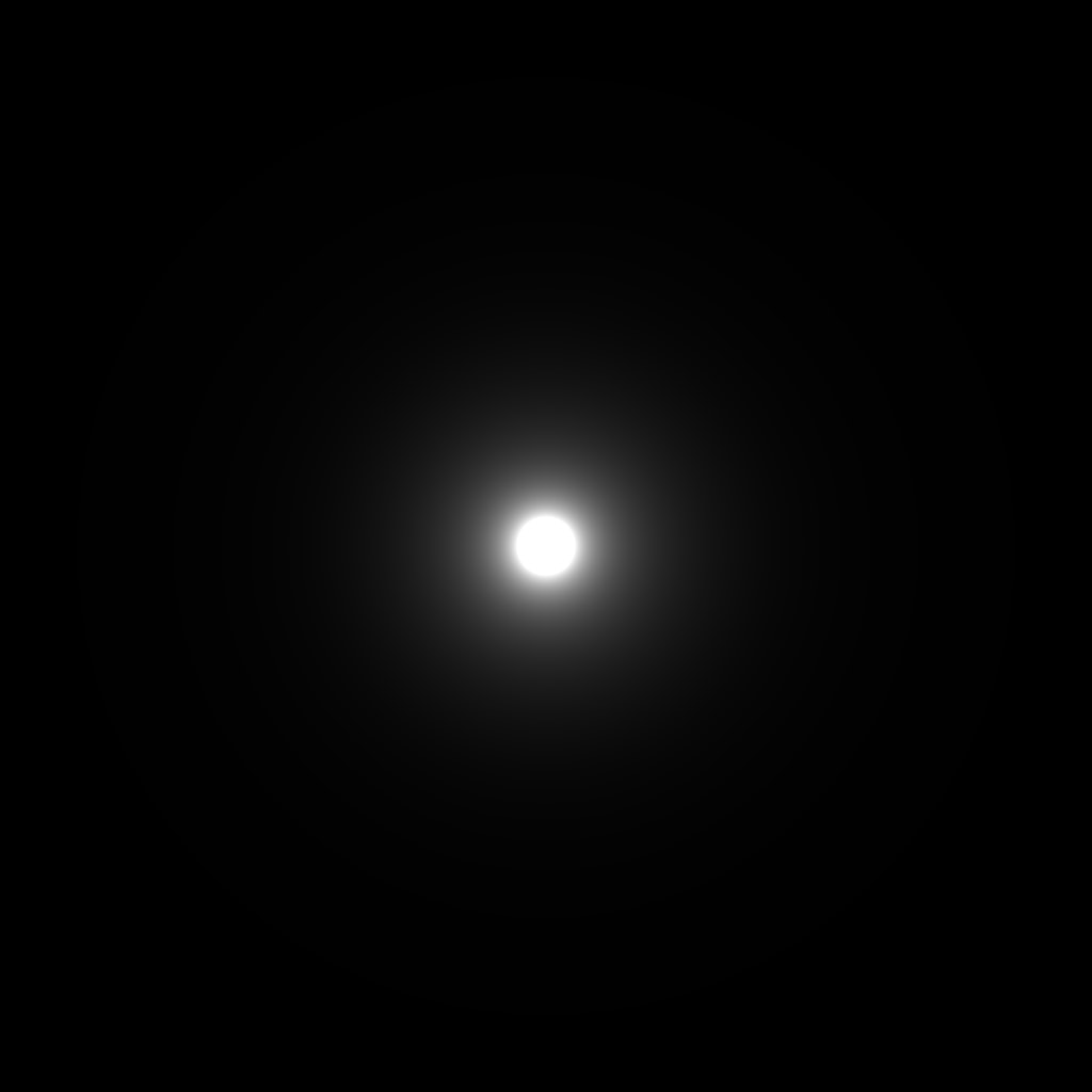
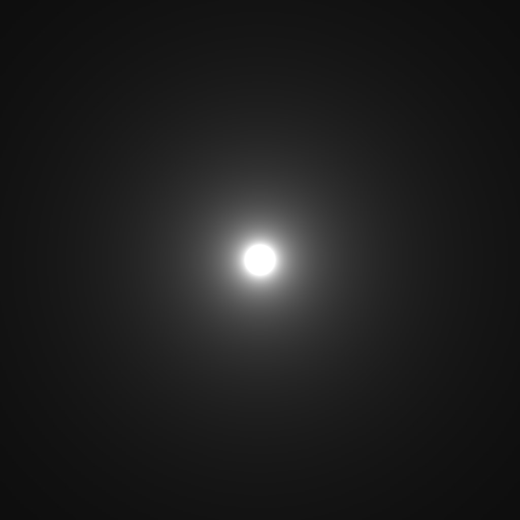
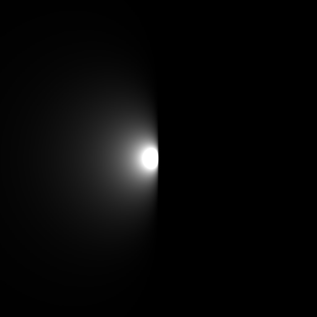
Here is the crop I'm interested in:

I wrote a Python script to read the pixel values in the center horizontal line of the image. It is using OpenCV, for EXR support (used later).

import cv2
import sys

img = cv2.imread(sys.argv[1], cv2.IMREAD_ANYCOLOR | cv2.IMREAD_ANYDEPTH)
assert img is not None

# sampling 8 rows at the center for smoothing
img_resized = cv2.resize(img, (img.shape[0], int(img.shape[1] / 8)), interpolation=cv2.INTER_AREA)

# if you want to see the image
# cv2.imshow('a', img_resized)
# cv2.waitKey(0)
# cv2.destroyAllWindows()

height, width, _ = img_resized.shape
half_height = int(height / 2)
half_width = int(width / 2)

values = []

for i in range(0, half_width):
    pixel = img_resized[half_height, i]
    y = (float(pixel[0]) + pixel[1] + pixel[2]) / 3
    x = 1 - (i / half_width)
    if 0.01 < x < 1:
        values.append((x, y))

# normalizing sampled max(y) to 1.0
y_max = max(y for _, y in values)
for x, y in values:
    y_mod = round(y / y_max, 3)
    print(f'{round(x, 3)},{y_mod}')

Copy and paste the values into Desmos Graphing Calculator.

Transforming between sRGB <> linear color space is done with ImageMagick:

convert srgb.png -colorspace sRGB -colorspace RGB linear.png

Checking curves

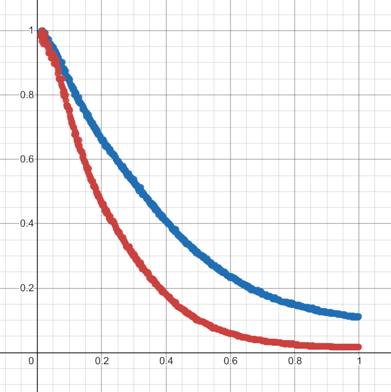
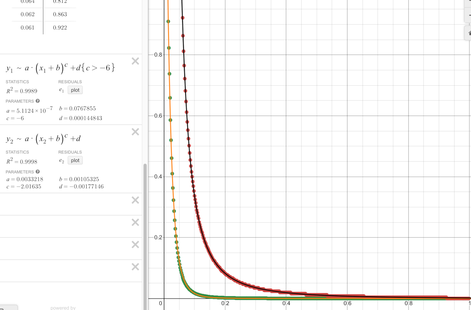
Desmos has an amazing curve-fitting / non-linear regression tool, let's see what kind of curve we can fit on our data.

Tried with power functions, didn't really work (look at the huge a at 10^12):

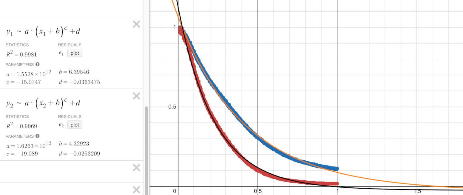
With exponential functions on the other hand it fits quite nicely:

Simulating the scene with Mitsuba

Mitsuba Renderer and PBRT are open-source Physically Based Renderers. They are considered the reference renderers for light calculations, for example, the Frostbite game engine used them for validating their Global Illumination models.

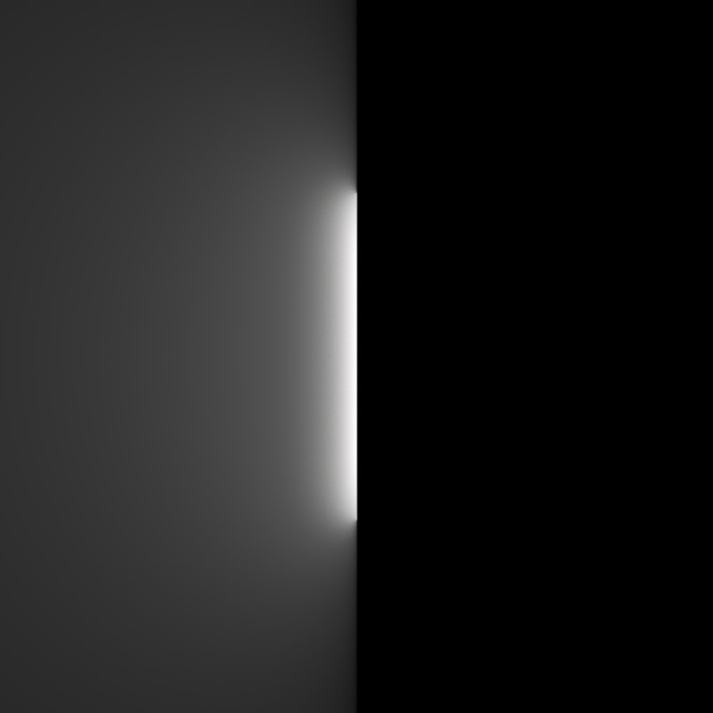
I made a basic scene in Mitsuba:

• matte floor plane (bsdf type="diffuse", spectrum name="reflectance" value="0.5")
• rectangle area emitter 1:10 aspect ratio, like 2 meter long, 20 cm high (emitter type="area", spectrum name="radiance" value="5"), touching the floor/

In 3D it looks like this:

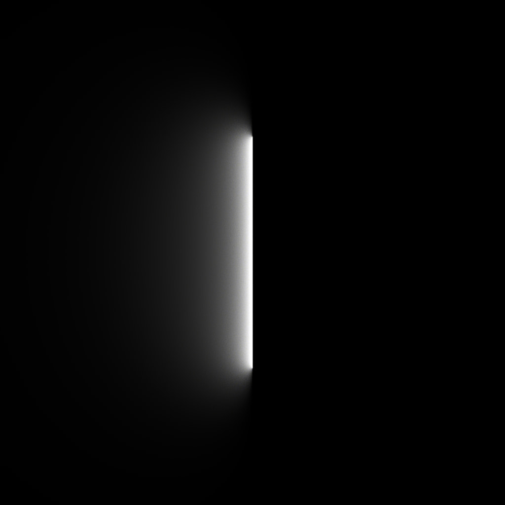
From a top view, it looks like this.

This looks nice, but a bit different compared to the iPhone wallpapers. Let's look at the curves.

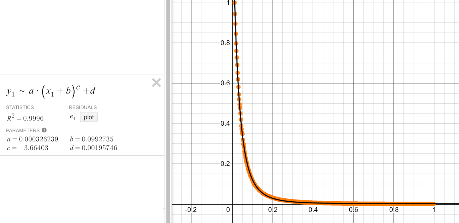
Interestingly, while the iPhone image had an exponential curve, the Mitsuba reference is close to a power function.

Tone mapping

Mitsuba exports a linear RGB HDR EXR file, not an SDR image, like a JPEG or PNG. To convert an EXR image to something we can display in a browser, we need to map it to the sRGB color space.
The simplest way to do this is to do the gamma correction, either with an imagemagick command like the one listed above or with a simple pow(col, 1/2.2) function. (sRGB is almost the same as gamma 2.2, and for our case with bright values, they are basically interchangeable). The rendered image above is converted using this simple gamma correction.

Applying the simple gamma correction is just one option. HDR to SDR tone mapping is a well-researched area with many algorithms. The open-source exrtools package has multiple methods for tone mapping EXR to sRGB. The package hasn't been updated since 2003, but fortunately, I found a Docker image, so it was quite simple to use it. I wrote exrtools.sh to run the reference examples.

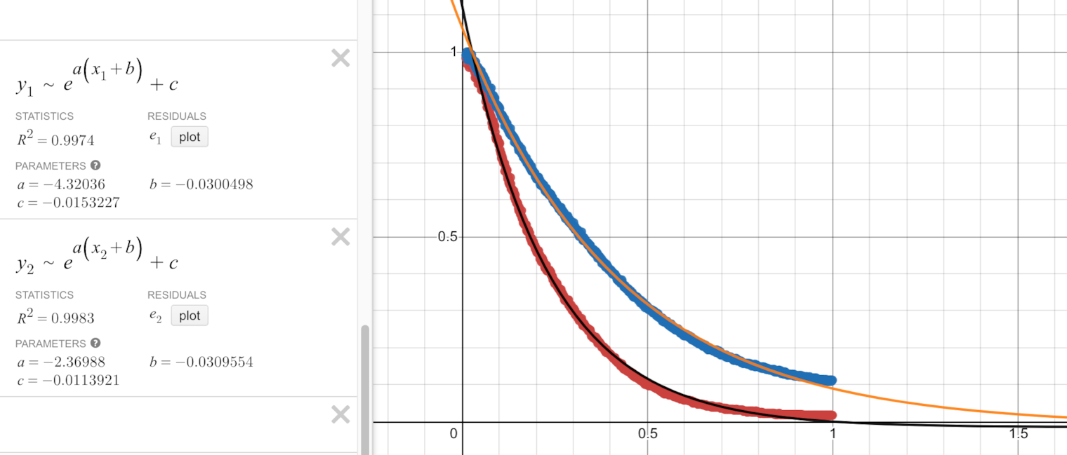
Let's have a look at the curves.

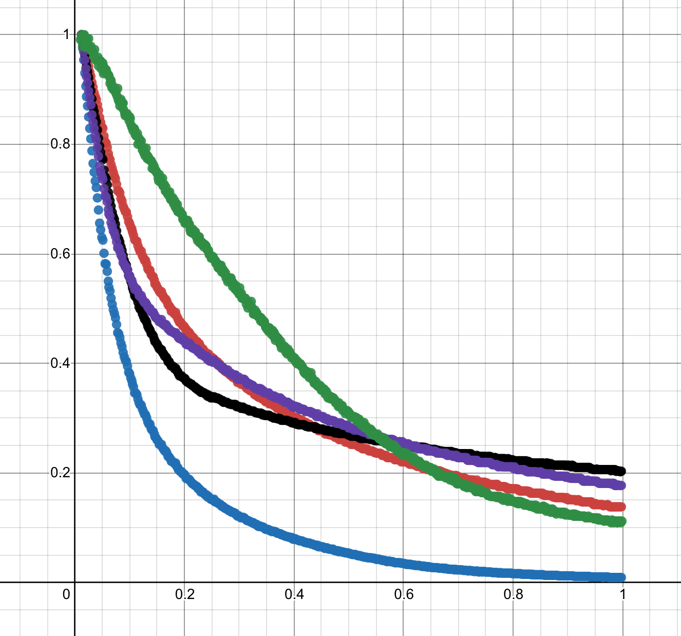
• Blue - simple gamma correction
• Red - photoreceptor physiology method
• Black - iCAM method
• Purple - non-linear masking method2
• Green - iPhone reference

Interesting, none of them looks like the reference image, but it is nice to see how tone mapping can change a scene.

Understanding area lights

Before understanding area lights, I need to understand their simpler counterparts:

• point lights
• "tiny disc" lights, which we can integrate over a rectangle to get to the area light

Point lights

Point lights are the simplest light sources to model, they radiate equally in all directions and follow the inverse square law.

I modified the previous Mitsuba scene to use a single point light, instead of the rectangle area light. The point light is 0.1 units above the ground plane (from top pixel to bottom pixel it is about 4 units.). Link to scene.xml.

To visualize the inverse square law, I made a shader on Shadertoy.com, the core of the shader being the following snippet:

float area_light_small(vec2 uv) {
	// could be optimised as dot(uv, uv)
  return 1. / (uv.x*uv.x + uv.y*uv.y);
}

Visually the shader looks a bit brighter, but looking at the curves, it's clear that they are very different. The Mitsuba one has \(\ x^{-6} \) falloff while the shader is \(\ x^{-2} \).

I suspect that the point light's "inverse square law" only applies to surfaces looking perpendicular to the light. Here, as we get further and further, the light arrives in a more and more shallow angle, thus giving us this effect.

The ground plane is an ideal 100% matte, perfect Lambertian surface. Lambert's cosine law states that "the radiant intensity ... observed from an ideal diffusely reflecting surface ... is directly proportional to the cosine of the angle θ between the direction of the incident light and the surface normal".

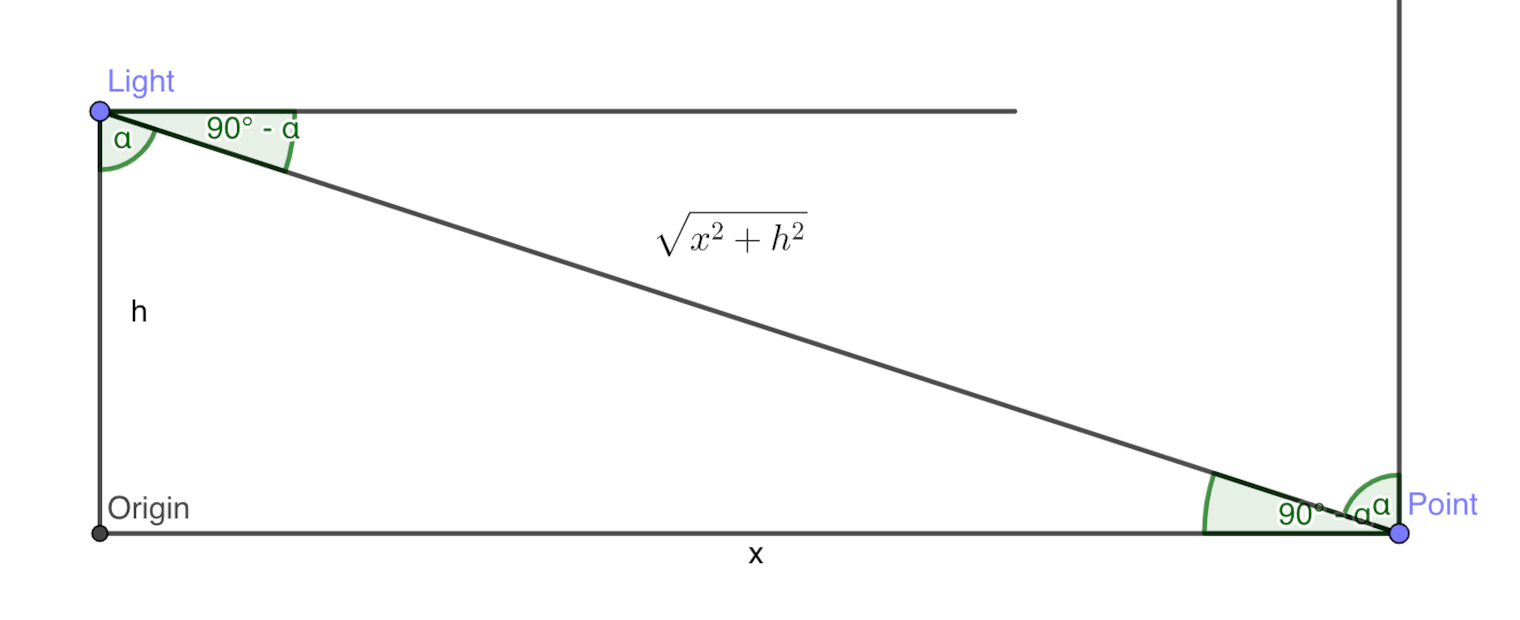
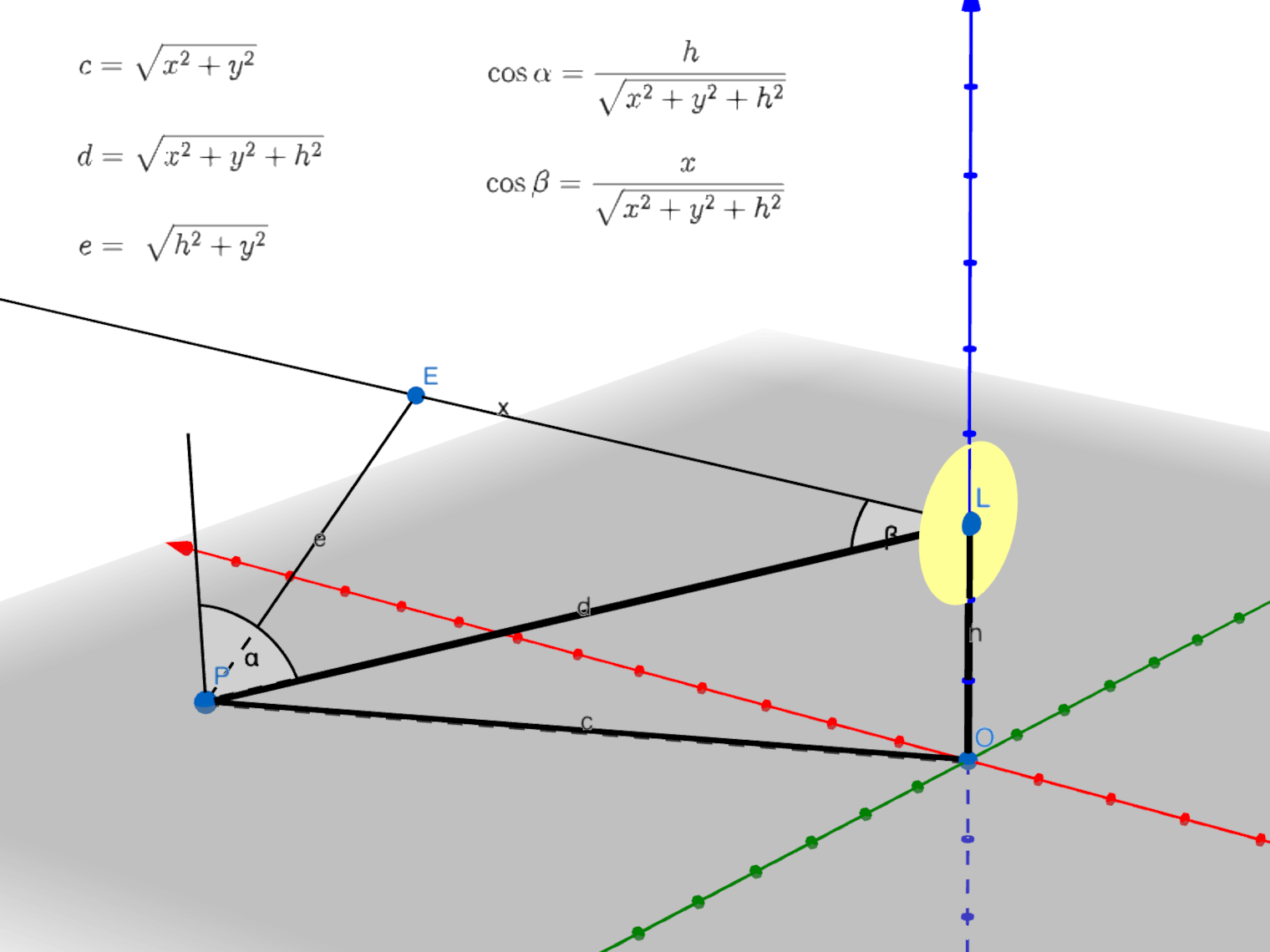
I made a sketch in GeoGebra to calculate the cosine we need. The point light is h unit above the origin, the tested point is at x position.

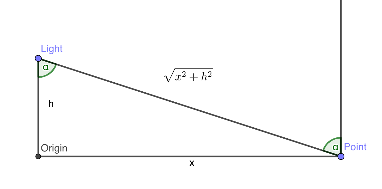
The Lambertian cosine is
$$ \cos(\alpha) = \frac{h}{\sqrt{x^2+h^2}} $$

The distance from the light is \(\sqrt{x^2+h^2}\)

Combining both, for a light h units above the ground, with i intensity is:

$$ f_{x} = \frac{h}{\sqrt{x^2+h^2}} \frac{i}{x^2+h^2} $$

Which can be simplified to:

$$ f_{x}\ = \frac{i\cdot h}{\left(x^{2}+h^{2}\right)^{\frac{3}{2}}} $$

or \(\ \frac{i\cdot h}{\sqrt{x^{2}+h^{2}}^{3}} \) where \(\ \sqrt{x^{2}+h^{2}} \) is the distance from the light.

Let's test this analytical solution by curve fitting:

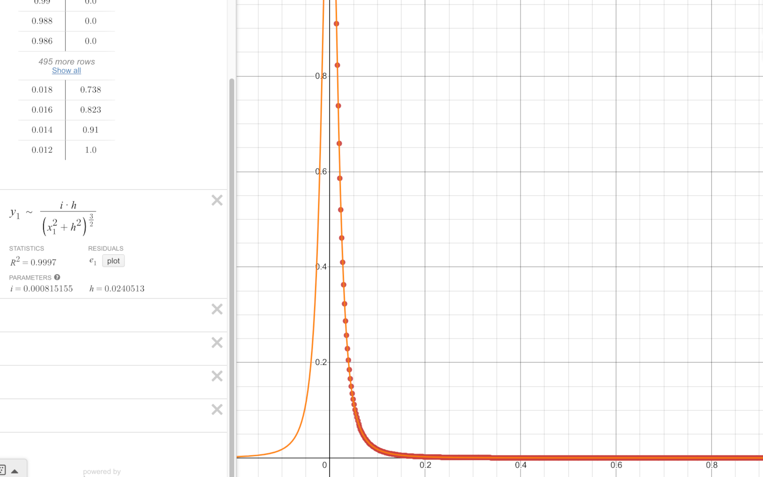
Perfect curve fitting, point light analytic solution found!

Shader

Physically correct point light shader:

float point_light(vec2 uv, float h, float i) {
  // h - light's height over the ground
  // i - light's intensity
  return i * h * pow(dot(uv,uv) + h*h, -1.5);
}

Interactive shader (press play button or open on Shadertoy):

"Tiny disc" light

The next step is to find the solution to a "tiny disc" light, which later we will integrate over a rectangle to get to the area light. Mitsuba scene.xml

This time, there is a Lambertian emitter (the light) and a Lamberian reflector (the ground plane), meaning we will have two cosine terms.

Simplified to y=0

Simplifying the case in 2D on the \(\ y=0 \) plane, we have:

$$ \cos\left(90-\alpha\right)\ =\ \sin\left(\alpha\right)\ =\frac{x}{\sqrt{x^{2}+h^{2}}} $$

Giving us:

$$ f_{x} = \frac{h}{\sqrt{x^{2}+h^{2}}}\cdot\frac{x}{\sqrt{x^{2}+h^{2}}}\cdot\frac{i}{x^{2}+h^{2}} = $$

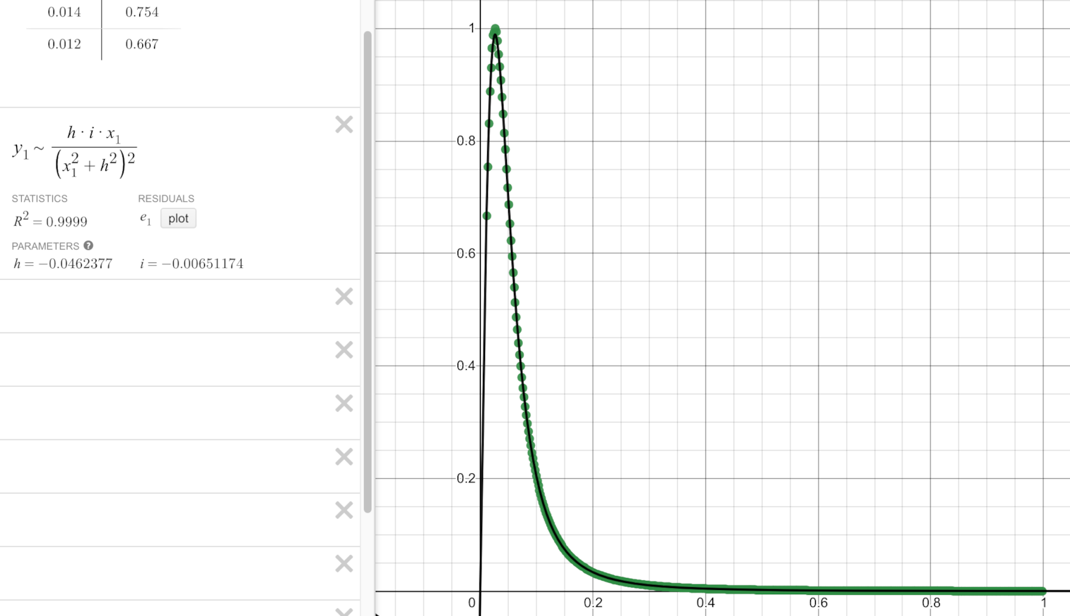
$$ = \frac{h\cdot i\cdot x}{\left(x^{2}+h^{2}\right)^{2}} $$

Testing curve fitting in Desmos gives us perfect fit!

General form in 3D

The next step is doing the calculation in 3D. Our point P lies on the ground plane, with\(\ x, y \) coordinates.

The "Lambertian cosine 1" * "Lambertian cosine 2" * falloff gives is the following equation:

$$ f_{x,y} = \frac{h}{\sqrt{x^{2}+y^{2}+h^{2}}}\cdot\frac{x}{\sqrt{x^{2}+y^{2}+h^{2}}}\cdot\frac{i}{x^{2}+y^{2}+h^{2}} = $$

$$ = \frac{h\ \cdot\ i\ \cdot\ x}{\left(x^{2}+y^{2}+h^{2}\right)^{2}} $$

Shader

Physically correct "tiny disc" light shader:

float disc_light(vec2 uv, float h, float i) {
  // h - light's height over the ground
  // i - light's intensity
  if (uv.x > 0.) return 0.;
  return i * h * -uv.x * pow(dot(uv,uv) + h*h, -2.);
}

Interactive shader (press play button or open on Shadertoy):

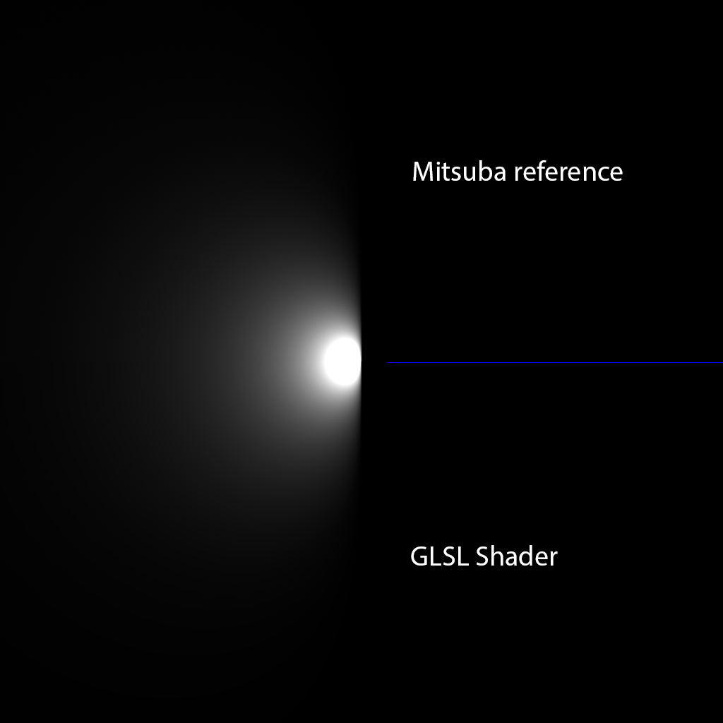
Validation

Comparing the Mitsuba reference EXR with the curve-fitted GLSL shader gives a close to perfect result. I'm honestly surprised it turned out so well.

Area light integration

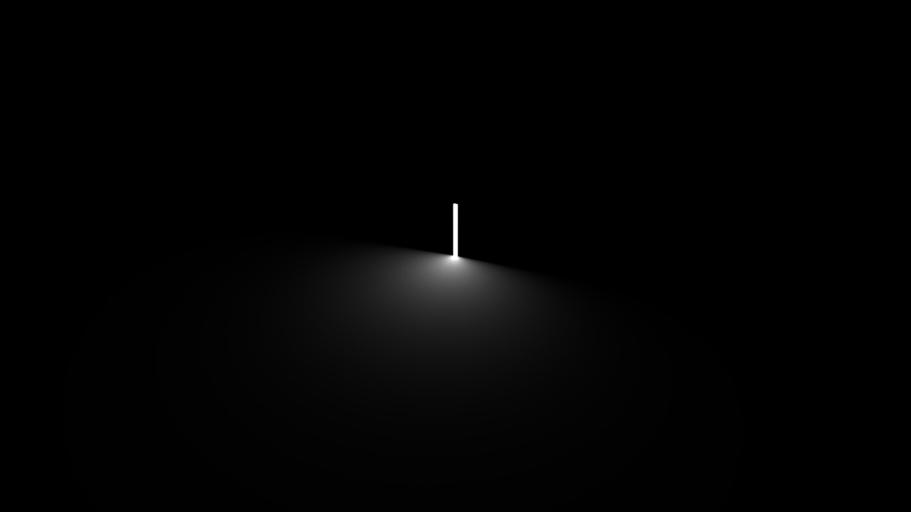
Point to line - "rod" light

First let's integrate the "tiny disc" light it over\(\ h \) so that it becomes a vertical "rod" light. The scene in 3D would look like the following:

For the calculation, integral-calculator.com helps us:

$$ \int\frac{\mathrm{i}xh}{\left(h^2+y^2+x^2\right)^2}dh = $$

$$ = -\dfrac{ix}{2\left(h^2+y^2+x^2\right)} $$

A shader for visual check:

float rod_light_antideriv(vec2 uv, float i, float h) {
  return i * uv.x / (dot(uv,uv) + h*h);
}

float rod_light(vec2 uv, float i, float h_top, float h_bottom) {
  // h_top and h_bottom - the light's top and bottom above the ground
  // i - light's intensity
  return rod_light_antideriv(uv, i, h_top) - rod_light_antideriv(uv, i, h_bottom);
}

Interactive shader (press play button or open on Shadertoy):

Line to rectangle - rectangle area lights

Now, let's make this "rod" light into a rectangle area light.

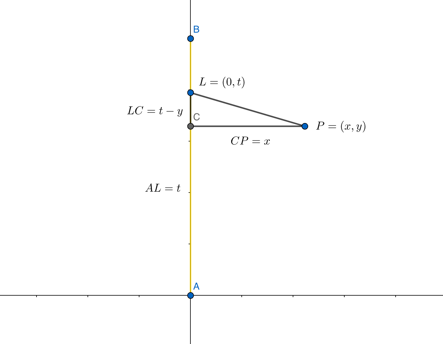
A "tiny disc" light\(\ L \) is on the y-axis, at\(\ L = (0, t) \) position. For a point\(\ P = (x, y) \), this light's contribution is:

$$ f_{x,y} = -\dfrac{ix}{2\left(h^2+(t-y)^2+x^2\right)} $$

Integrating it over\(\ t \), gives us the antiderivative:

$$ \int-\dfrac{ix}{2\left(\left(t-y\right)^2+x^2+h^2\right)}dt = $$

$$ = -\dfrac{ix\arctan\left(\frac{y-t}{\sqrt{x^2+h^2}}\right)}{2\sqrt{x^2+h^2}} $$

The final area light shader

A shader based on this function:

float area_light_antideriv(vec2 uv, float i, float h, float t) {
  float lxh = length(vec2(uv.x, h));
  return -i * uv.x * atan((t-uv.y)/lxh) / lxh;
}

float area_light(vec2 uv, float i, float h_bottom, float h_top, float t_start, float t_end) {
  // i - light's intensity
  // h_top and h_bottom - the light's top and bottom above the ground
  // t_start and t_end - the light's start and end on the y-axis
  float v =
  + area_light_antideriv(uv, i, h_top, t_end)
  + area_light_antideriv(uv, i, h_bottom, t_start)
  - area_light_antideriv(uv, i, h_bottom, t_end)
  - area_light_antideriv(uv, i, h_top, t_start);
  return max(0., v);
}

Interactive shader (press play button or open on Shadertoy):